Log & Power-Law (Gamma) Transformations

Theory

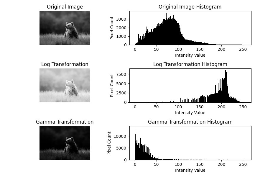
Non-linear intensity transformations are used to enhance the contrast and brightness of an image in a non-linear fashion. These transformations map input intensity values to output values according to logarithmic or power-law functions.

1. Logarithmic Transformation

The logarithmic transformation enhances the intensity of dark regions in an image while compressing the brighter regions. It is defined as:

s = c * log(1 + r)

where r is the input pixel intensity, s is the output intensity, and c is a scaling constant.

2. Power-Law (Gamma) Transformation

Power-law transformations adjust image brightness using a gamma value:

s = c * r^γ

• γ < 1: Brightens the image
• γ = 1: Linear mapping
• γ > 1: Darkens the image

3. Applications

• Enhancement of satellite and medical images
• Correction of illumination issues
• Preprocessing for computer vision tasks

Python Code

import cv2
import numpy as np
import matplotlib.pyplot as plt

# Load grayscale image
img = cv2.imread('assets/bear.jpg', cv2.IMREAD_GRAYSCALE)

# Log Transformation
c_log = 255 / np.log(1 + np.max(img))
log_transformed = c_log * np.log(1 + img)
log_transformed = np.uint8(log_transformed)

# Gamma Transformation
gamma = 2.2  # try values like 0.5, 1.5, 2.0
c_gamma = 255 / (np.max(img) ** gamma)
gamma_transformed = c_gamma * (img ** gamma)
gamma_transformed = np.uint8(gamma_transformed)

# Display images with histograms
images = [img, log_transformed, gamma_transformed]
titles = ['Original Image', 'Log Transformation', 'Gamma Transformation']

plt.figure(figsize=(10, 6))
for i in range(3):
    # Image
    plt.subplot(3, 2, i*2 + 1)
    plt.imshow(images[i], cmap='gray')
    plt.title(titles[i])
    plt.axis('off')

    # Histogram
    plt.subplot(3, 2, i*2 + 2)
    plt.hist(images[i].ravel(), bins=256, range=(0, 256), color='black')
    plt.title(f"{titles[i]} Histogram")
    plt.xlabel("Intensity Value")
    plt.ylabel("Pixel Count")

plt.tight_layout()
plt.show()
        

Example Output