Histogram Analysis

Theory

A histogram is one of the most fundamental tools in image processing. It provides a graphical representation of pixel intensity distribution, allowing us to analyze how brightness and contrast are spread across an image.

1. Understanding Brightness and Contrast

A histogram shows how many pixels fall into each intensity level (0–255 for 8-bit images). A narrow histogram may indicate low contrast, while a wider spread suggests higher contrast.

2. Detecting Exposure Issues

• If values cluster on the left → the image is likely underexposed (too dark).
• If values cluster on the right → the image may be overexposed (too bright).

3. Enhancing Images with Histograms

Histogram-based methods like contrast stretching and histogram equalization adjust pixel intensities to improve image quality. These are widely used in medical imaging, satellite imaging, and photography.

4. Grayscale vs. Color Histograms

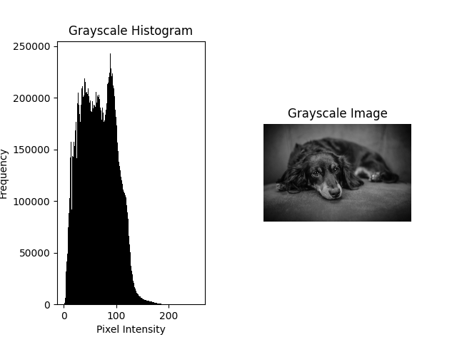
• Grayscale histograms focus on intensity values from a single channel.
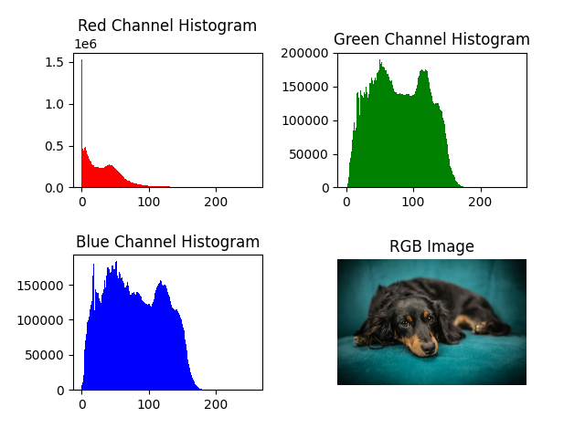
• Color histograms are computed separately for Red, Green, and Blue channels, useful for analyzing color balance and detecting artifacts.

In short, histogram analysis helps us diagnose image quality, detect exposure problems, and prepare images for advanced processing tasks like segmentation and enhancement.

Python Code

import cv2
import numpy as np
import matplotlib.pyplot as plt

def plot_histogram(image, color_space="BGR"):
    """
    Plot histograms for grayscale or color images.
    """
    if color_space == "GRAY":
        # Grayscale histogram
        plt.subplot(1, 2, 1)
        plt.hist(image.ravel(), bins=256, range=[0, 256], color="black")
        plt.title("Grayscale Histogram")
        plt.xlabel("Pixel Intensity")
        plt.ylabel("Frequency")

        plt.subplot(1, 2, 2)
        plt.imshow(image, cmap="gray")
        plt.title("Grayscale Image")
        plt.axis("off")

        plt.subplots_adjust(hspace=0.4, wspace=0.4)
        plt.show()

    elif color_space == "BGR":
        # Convert BGR → RGB for correct color display
        image_rgb = cv2.cvtColor(image, cv2.COLOR_BGR2RGB)

        plt.subplot(2, 2, 1)
        plt.hist(image[:, :, 2].ravel(), bins=256, range=[0, 256], color="r")
        plt.title("Red Channel Histogram")

        plt.subplot(2, 2, 2)
        plt.hist(image[:, :, 1].ravel(), bins=256, range=[0, 256], color="g")
        plt.title("Green Channel Histogram")

        plt.subplot(2, 2, 3)
        plt.hist(image[:, :, 0].ravel(), bins=256, range=[0, 256], color="b")
        plt.title("Blue Channel Histogram")

        plt.subplot(2, 2, 4)
        plt.imshow(image_rgb)
        plt.title("RGB Image")
        plt.axis("off")

        plt.subplots_adjust(hspace=0.5, wspace=0.4)
        plt.show()

# Load an image
image_path = "assets/dog.jpg"
image = cv2.imread(image_path)

if image is None:
    print("Error: Image not found!")
    exit()

# Convert to grayscale
gray_image = cv2.cvtColor(image, cv2.COLOR_BGR2GRAY)

# Plot histograms
plot_histogram(gray_image, color_space="GRAY")
plot_histogram(image, color_space="BGR")
        

Output Example

Below are example histograms for a grayscale and color image: